Kalman Filter¶

The Kalman Filter is used for prediction and estimation of the state of a system. The Kalman filter requires two models: the state model and the observation model.

State Model : A model that represents changes in the state of the system with respect to time.
Observation Model : An equation/model that represents data measured, usually by sensors, providing external data about the robot and linking it to the system's state.

Multivariate Kalman Filter¶

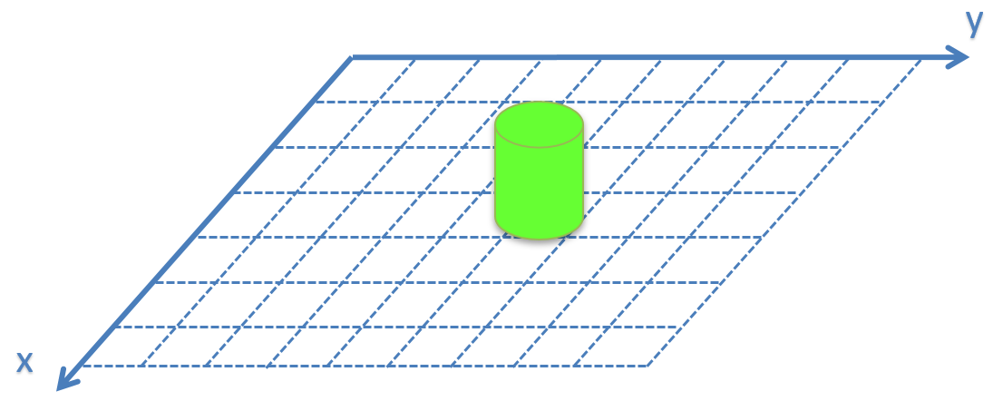
The system state is represented as:

\[ \textbf{x} = \begin{bmatrix} x \\ y \end{bmatrix} \]

Multivariate Kalman Filter produces outputs in the form of multivariate random variables and a covariance matrix, which is a square matrix representing the uncertainty of the states. The Covariance matrix in the Kalman Filter includes:

\(P_{n,n}\): covariance matrix for estimation
\(P_{n+1,n}\): covariance matrix for prediction
\(R_n\): covariance matrix representing measurement uncertainty
\(Q\): covariance matrix for process noise

Covariance¶

Covariance measures the correlation between two or more random variables.

Object on the x-y plane

Covariance between population \(X\) and \(Y\), with \(N\) data points:

\[ COV(X, Y) = \frac{1}{N}\sum_{i=1}^N(x_i - \mu_x)(y_i-\mu_y) \]

For a sample:

\[ COV(X, Y) = \frac{1}{N-1}\sum_{i=1}^N(x_i - \mu_x)(y_i-\mu_y) \]

Covariance Matrix¶

The covariance matrix is a square matrix representing the covariance between each element of each state.

\[ \Sigma = \begin{bmatrix} \sigma_{xx} & \sigma_{xy} \\ \sigma_{yx} & \sigma_{yy} \end{bmatrix} = \begin{bmatrix} \sigma_{x}^2 & \sigma_{xy} \\ \sigma_{yx} & \sigma_{y}^2 \end{bmatrix} = \begin{bmatrix} VAR(x)& COV(x,y) \\ COV(y,x) & VAR(y) \end{bmatrix} \]

If \(x\) and \(y\) are uncorrelated, the off-diagonal elements of the matrix \(\Sigma\) are zero.

For a state \(x\) of dimension \(1 \times k\):

\[ COV(x) = E((x-\mu_x)(x-\mu_x)^T) \]

Proof :

\[ \begin{align*} COV(x) &= E \left( \begin{bmatrix} (x_1 -\mu_{x_1})^2 & (x_1-\mu_{x_1})(x_2-\mu_{x_2}) & \cdots &(x_1-\mu_{x_1})(x_k-\mu_{x_k})\\ (x_2-\mu_{x_2})(x_1 -\mu_{x1}) & (x_2-\mu_{x_2})^2 & \cdots &(x_2-\mu_{x_1})(x_k-\mu_{x_k})\\ \vdots & \vdots & \ddots & \vdots \\ (x_k-\mu_{x_k})(x_1 -\mu_{x1}) & (x_k-\mu_{x_k})(x_2-\mu_{x_2}) & \cdots &(x_k-\mu_{x_k})^2\\ \end{bmatrix} \right)\\ &= E \left( \begin{bmatrix} (x_1 -\mu_{x_1})\\ (x_2-\mu_{x_2})\\ \vdots \\ (x_k-\mu_{x_k}) \end{bmatrix} \begin{bmatrix}(x_1 -\mu_{x_1})&(x_2-\mu_{x_2})&\cdots & (x_k-\mu_{x_k}) \end{bmatrix} \right)\\ & = E((x_{1:k}-\mu_{x_{i:k}})(x_{1:k}-\mu_{x_{i:k}})^T) \end{align*} \]

Note :

\(E(v)\) is the expectation or mean of the random variable.

Covariance Matrix Properties¶

\[ \begin{align} \Sigma_{ii} = \sigma_{ii}^2\\ tr(\Sigma) = \sum _{i=1}^n \Sigma_{ii}\geq 0\\ \Sigma = \Sigma^T\\ \end{align} \]

Multivariate Gaussian Distribution¶

\[ p(x|\mu, \Sigma) = \frac{1}{\sqrt{(2\pi)|\Sigma|}}exp\left (-\frac{1}{2}(x-\mu)^T \Sigma^{-1}(x-\mu)\right ) \]

State Equation¶

State Equation Used to make predictions based on existing estimates.

\(\hat{x}_{n+1,n} = F\hat{x}_{n,n} + G\hat{u}_{n,n} +w_n\)

\(\hat{x}_{n+1,n}\) : predicted state at \(n+1\)
\(\hat{x}_{n,n}\) : predicted state at \(n\)
\(u_n\) : control input measured into the system
\(w_n\) : noise, unmeasured input (called process noise)
\(F\) : transition matrix
\(G\) : control matrix (mapping the effect of \(u_n\) to the state variables)

Covariance Equation¶

Measures the uncertainty of predictions made by the State Equation

\(P_{n+1,n} = FP_{n,n}F^T + Q\)

Proof :

Using \(COV(x) = E((x_{1:k}-\mu_{x_{i:k}})(x_{1:k}-\mu_{x_{i:k}})^T)\), then \(P_{n,n} = E((\hat{x}_{n,n}-\mu_{\hat{x}_{n,n}})(\hat{x}_{n,n}-\mu_{\hat{x}_{n,n}})^T)\)

From the state equation, \(P_{n+1,n}\) is derived as:

\[ \begin{align} P_{n+1,n} &= E((\hat{x}_{n+1,n}-\mu_{\hat{x}_{n+1,n}})(\hat{x}_{n+1,n}-\mu_{\hat{x}_{+1,n}})^T)\\ &= E \left ( (F\hat{x}_{n,n} + G\hat{u}_{n,n} - F\hat{\mu_x}_{n,n} + G\hat{u}_{n,n}) (F\hat{x}_{n,n} + G\hat{u}_{n,n} - F\hat{\mu_x}_{n,n} + G\hat{u}_{n,n})^T \right )\\ &=E \left(F(\hat{x}_{n,n} - \mu_{x_{n,n}}) (F(\hat{x}_{n,n} - \mu_{x_{n,n}}))^T\right)\\ &=E \left(F(\hat{x}_{n,n} - \mu_{x_{n,n}}) (\hat{x}_{n,n} - \mu_{x_{n,n}})^T F^T\right)\\ &=FE \left[(\hat{x}_{n,n} - \mu_{x_{n,n}}) (\hat{x}_{n,n} - \mu_{x_{n,n}})^T\right]F^T\\ \end{align} \]

Thus,

\[ \begin{align} P_{n+1,n} &= FP_{n,n}F^T \end{align} \]

Observation Model¶

\(z_n = Hx_n+v_n\)

\(z_n\) : observation vector
\(H\) : observation matrix
\(x_n\) : true state
\(v_n\) : random noise (called observation noise)

For example, in the case of an ultrasonic distance sensor, where the system state is the distance \(x_n\) and the sensor output is the measured ToF \(z_n\)::

\(z_n = [\frac{2}{c}]x_n + v_n\)

Where \(c\) is the speed of sound.

Observation Uncertainty¶

\(R_n = E(v_nv_n^T)\)

\(R_n\): covariance matrix for observation
\(v_n\): observation error

Process Uncertainty¶

\(Q_n = E(w_nw_n^T)\)

\(Q_n\): covariance matrix for process noise
\(w_n\): process noise

Summary¶

The Kalman Filter Diagram

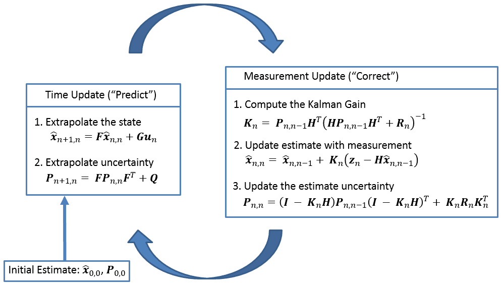
Kalman Gain¶

Kalman Gain determines the weighting for the measurement model. It defines the influence of the measurement model on state estimation:

\[ KG = \frac{error_{estimate}}{error_{estimate} + error_{measurement}} \]

If \(error_{estimate} > error_{measurement}\), then \(KG \rightarrow 1\)
If \(error_{estimate} < error_{measurement}\), then \(KG \rightarrow 0\)

\[ estimate_t = estimate_{t-1} + KG(measurement_t-estimate_{t-1}) \]

Error on Estimation¶

\[ E_{estimate_t} = [1-KG]E_{estimate_{t-1}} \]

If \(KG\rightarrow1\), the error on the estimation is large, resulting in a smaller \(E_{estimate}\).
If \(KG\rightarrow0\), the error on the estimation is small, maintaining the estimation error from time \(t-1\). Thus,
\(E_{estimate_t} < E_{estimate_{t-1}}\)

Note: As the estimation variance decreases, it approaches the true value.